Carlistle 2005 urban flooding

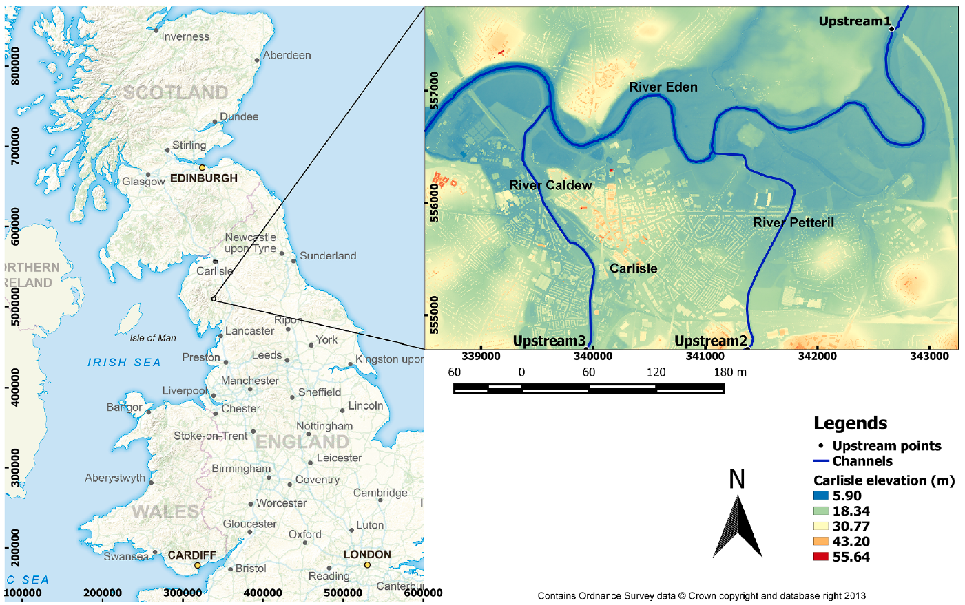
This test case is aimed to simulate urban flooding over a real-world study area, where the flooding occurs from three inflow sources. It is useful to understand how to handle multiple point source inflow boundary conditions in LISFLOOD-FP. The study area is about 14.5 square kilometres and includes the urban area of Carlisle, a city in northern England with a population of 70,000 that was heavily hit by flooding in January 2005 (Horritt et al., 2010). The flooding hydrodynamics was driven by three river streams: River Eden, River Petteril and River Caldew, located within the study area. The figure below shows the study area and the three locations, Upstream 1, Upstream 2 and Upstream 3, for each of the river streams from where the flood flow occurred.

To apply LISFLOOD-FP to simulate the 2005 flooding event, the DEM data and the three upstream inflow boundary conditions are required. A 5 m x 5 m resolution DEM data, named carlisle-5m.dem, was obtained from the School of Geographical Sciences at the University of Bristol. It was created by further processing the LiDAR DEM provided by the UK Environment Agency (EA) by removing the noises and obstacles (e.g. trees and bridges). A uniform Manning coefficient of 0.055 is specified for the whole domain.

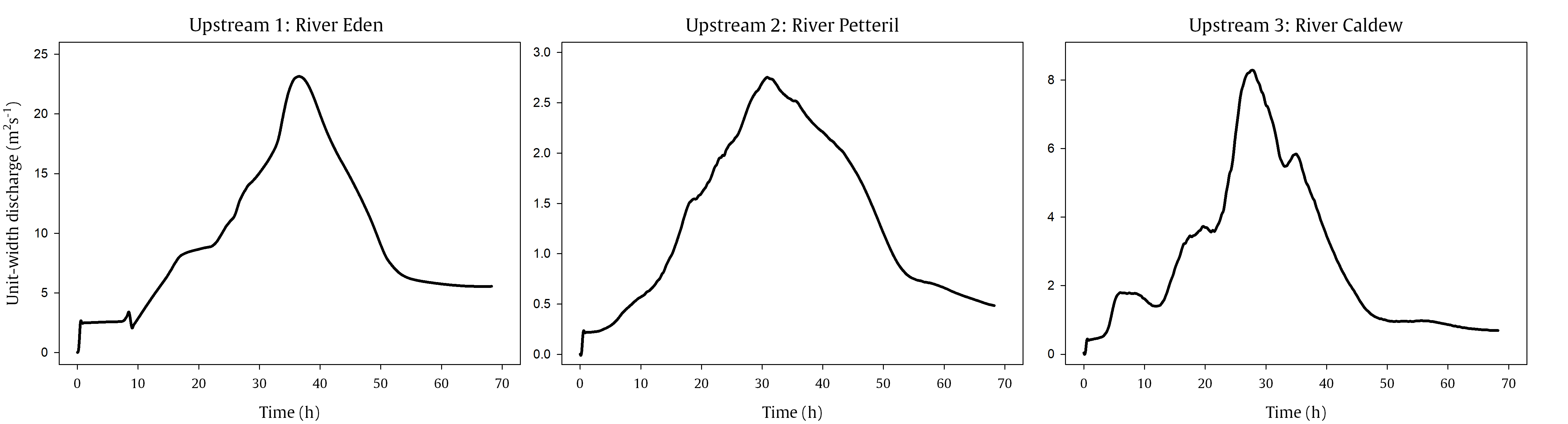
Floodwater flow breached from the three openings, Upstream 1, Upstream 2 and Upstream 3, based on three different discharge hydrographs (in 15-minute intervals). These hydrographs are shown in the figure below. They were generated through 1D flood routing from previous studies (e.g. Neal et al. (2013)).

To set up LISFLOOD-FP, starting from carlisle-5m.bci, the discharge (inflow) hydrographs have to be specified as point sources (inflow boundary conditions), while the western edge of the study area is set to allow free outflow of the water. The figure below shows a screenshot of the carlisle-5m.bci file.

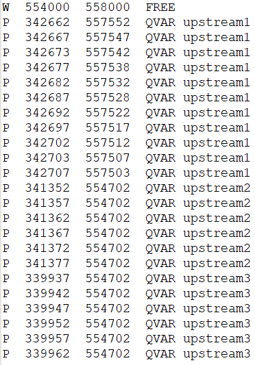
The first row includes the W identifier for activating the west boundary as FREE outflow condition, between the locations defined by the two Y-direction coordinates listed in the second and third columns. The following rows specify a series of points sources (identifier P), defined as the time-varying inflow (type QVAR) with names upstream1, upstream2, upstream3. Note that these names must be consistent with the naming of the time series specified in the .bdy, explained below.

For the 5 m × 5 m resolution DEM data, 11 cells span the upstream1 time series to cover the width of River Eden from point (x,y) = (342662, 557552) to (x,y) = (342707, 557503), 6 cells span the upstream2 time series to cover the width of River Petteril from point (x,y) = (341352, 554702) to (x,y) = (341377, 554702), and 6 cells span the upstream3 time series to cover the width of River Caldew from point (x,y) = (339937, 554702) to (x,y) = (339962, 554702). For the DEM data files with a finer or coarser resolution, different numbers must be specified by manually investigating the positions via QGIS.

The time-varying inflows, upstream1, upstream2 and upstream3, specified in the carlisle-5m.bci file must be provided in a time series file, named carlisle.bdy file. The layout of the carlisle.bdy file is similar to the one explained for “Valley flooding” test case. However, for this test case, the .bdy file must include the three time series, listed one after another. For the first time series, the name upstream1 must be specified followed by the number of time intervals and the lists of the time-varying inflow discharge, alongside its time of occurence. The second time series, with the name upstream2, and then the third time series, with the name upstream3, are handled similarly.

All the input files required to run the simulations are provided for UoS users in the testing\UoS\T07 directory of LISFLOOD-FP-trunk repository, and for external users in Data\T07 (recall “Input files and their format”). The 68-hour long simulations are run with the ACC, FV1 and DG2 solvers, all on the same 5 m × 5 m resolution grid.

Once the simulations are done, a set of output files are generated, including the water depth or velocity stage files and water depth and maximum water depth 2D maps (recall “Running the code, outputs and visualisation”). To analyse the outputs of a simulation (or “model data”), they often get compared to the reference (or “benchmark data”). When considering the free-surface elevation (or water depth or velocity) at a stage point, the benchmark data are usually the predictions from another simulation (e.g. using a more accurate solver), or in-situ observations (if available). The model and benchmark data at the stage points are often compared based on metrics like RMSE (root-mean-square error) or the bias (mean difference) (Hoch and Trigg, 2019).

From a practical point of view, one may be interested to analyse “flood extent” outputs of a flood modelling simulation, for example by taking the flood extent predicted by the ACC solver to be the model data to evaluate the flood extent predicted by the DG2 solver, considered as the benchmark data. With LISFLOOD-FP, the flood extent of a simulation is recorded in the .max file generated at the end of each simulation (recall “Running the code, outputs and visualisation”). The figure below shows the model and benchmark data for Carlisle 2005 flooding test case.

To compare two sets of flood extent maps, three metrics are commonly used (Wing et al., 2017): the Hit Rate (H), the False Alarm Ratio (F), and the Critical Success Index (C). To compute these three metrics, a post-processing toolkit, named metrics.py, is provided in the postprocess directory of LISFLOOD-FP-trunk repository. The definition of these metrics and how to use the toolkit to generate them are described in “Metrics for comparing two different flood extent predictions”.

Applying the toolkit to the two flood extent maps of the model and benchmark data outputs the following metrics:

Hit rate: 0.905324
False Alarm rate: 0.026091
Critical success index: 0.883887

A contingency map is also saved, as shown in the figure below.

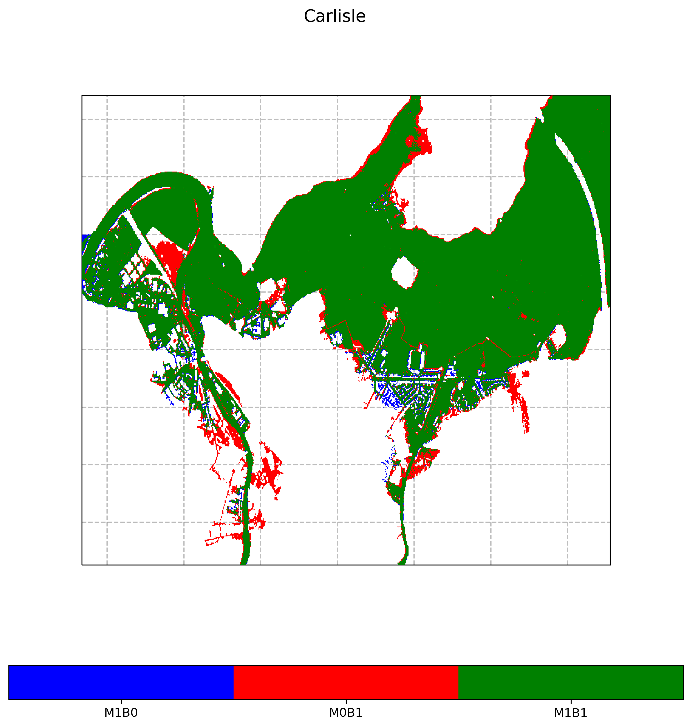
The combination of the metrics and the contingency map provides a measure on how much and in which areas the benchmark and model flood extents differ or agree. In this example, the hit rate of 0.90 indicates that 90% of the benchmark flood extent is also covered by the model flood extent. These areas are shown in green on the contingency map. In other words, only 10% of the benchmark flood extent is missed by the model, as shown in red on the contingency map.

The false alarm ratio of 0.02 shows that only 2% of the model flood extent is outside of the benchmark flood extent. These areas are shown in blue on the contingency map.

The critical success index of 0.88 shows that 88% of the whole flood extent is correctly covered by the model extent. In this sense, the whole flood extent is the union of three areas: (i) the area correctly covered by the model extent, (ii) the area missed by the model extent and (iii) the area of the model extent that is outside of the benchmark extent.

back