SEAMLESS-WAVE

SEAMLESS-WAVE is a developing “SoftwarE infrAstructure for Multi-purpose fLood modElling at variouS scaleS” based on "WAVElets" and their versatile properties. The vision behind SEAMLESS-WAVE is to produce an intelligent and holistic modelling framework, which can drastically reduce iterations in building and testing for an optimal model setting, and in controlling the propagation of model-error due to scaling effects and of uncertainty due statistical inputs.
Valley flooding following a dam failure
This test case is standard to study and compare the capabilities of 2D hydrodynamic solvers for modelling rapidly-propagating flow over a non-smooth valley (Ayog et al., 2021; Shaw et al., 2021). The 10 m × 10 m resolution DEM and the inflow hydrograph are available from the UK Environment Agency. Coarser resolution DEMs can be produced via QGIS (recall the “Preparing the input data” section in Merewether case study).
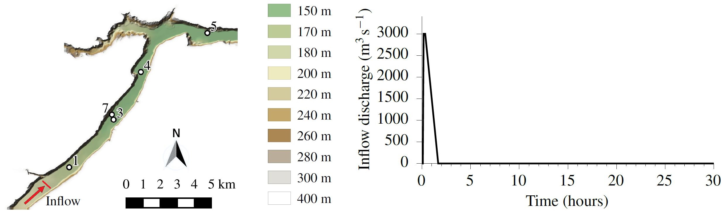
Flooding occurs from an opening located inside the valley from the southwest side (see the left panel in the figure above) where a strong inflow peak occurs (see the right panel in the figure). The inflow hydrograph is featured by a discharge of 3000 cubic metres per second occurring during t = 600 to 1200 seconds. This causes a flash flood propagation throughout the valley until after 30 hours when the water has ponded near the closed boundary at the eastern edge of the domain. A uniform Manning coefficient of 0.04 is specified for the whole domain.
To set up this test case, a point source boundary condition is required. This type of boundary condition is defined by specifying the inflow at certain locations inside the domain. Since maximum one point source is allowed per computational cell, the number of point sources depends on the resolution of the grid.
For this test case, the opening for the inflow is located along a line extending from point (x,y) = (232595, 830480) to (x,y) = (232785, 830290). By opening the DEM file, namely, ea5-10m.dem, in QGIS, it can be observed that the line spans 20 cells inside the domain for the 10m-resolution grid. The locations of these 20 cells along with Boundary identifier (P for point source), Boundary condition type (QVAR for time-varying inflow) and Boundary condition time series name (here named test5) must be provided in the .bci file, as shown in the screenshot below (details in “Boundary condition type file (.bci)”).
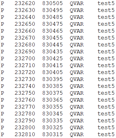
If a different grid resolution is to be used, it is necessary to re-check, manually (e.g. using QGIS), which are the cells spanning the length of the inflow opening and list them in the .bci file.
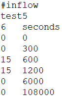
When a time-varying inflow is specified in a .bci file, it should be accompanied by a .bdy file that includes the Boundary condition time series name (test5 for this test case) in the first row. The second row should include the number of time intervals (6 for this test case) and the unit of time (seconds for this test case). The rest of the rows lists the time-varying inflow discharge (first column) alongside its time of occurence (second column). The inflow data between these intervals will be linearly interpolated by LISFLOOD-FP. The inflow (discharge) data must be provided in terms of unit-width discharge, q = Q/B.
The figure below shows a screenshot of the .bdy file for this test case, named ea5.bdy. It provides the time series of the unit-width discharge. Since the inflow starts at t = 300s, zero discharge is specified during the t = 0 to 300 seconds interval in the time series. The discharge reaches the peak of 3000 cubic metres per second at t = 600s and stays at the peak until t = 1200 seconds. This peak discharge is converted to unit-width discharge based on the discrete length of the opening for the 10m-resolution grid, spanning the 20 cells of length 10 m each, i.e. leading to q = Q/B = 3000/(20 x 10) = 15. At t = 1200s, the inflow decreases to reach zero at t = 6000 seconds after which a zero discharge is specified.
All the input files required to run the simulations are provided for UoS users in the testing\UoS\T06 directory of LISFLOOD-FP-trunk repository, and for external users in Data\T06 (recall “Input files and their format”). The simulations are run using the ACC, FV1 and DG2 solvers. The simulated values of the free-surface elevation (in metre) and velocity (in metre per second) are extracted at the stage points 1 to 7 (recall “Running the code, outputs and visualisation”), with the locations shown in the DEM figure at the beginning of this page.
The upper panels of the figure below show the free-surface elevations at points 1, 3, 5 and 7. The results show negligible differences in the free-surface elevations predicted by the three solvers. The predictions are also in close agreement with those resulted from the existing industrial models (e.g. Fig. 4.16 in Néelz and Pender (2013)).
The lower panels of the figure show the velocities at points 1, 3, 4 and 7. Bigger differences are found in velocity predictions. In particular, the ACC solver overpredicts the peak velocities at points 1, 4 and 7, which might be related to the fact that the local inertia formulation of the ACC solver is not physically valid for modelling abrupt changes in water depth (Shaw et al., 2021). The predictions by the FV1 solver are, however, in a closer agreement with the ones from the DG2 solver.
